The time of artificial intelligence has finally arrived. Although AI had its emergence as a field of study since the late 60s, it remained on the margins as more of a research area with little or no actual impact on mainstream real-world problem solving.
The advent of affordable and prevalent high compute hardware, coupled with parallel processing with emerging platforms such as cloud-based infrastructure, has made it possible to deploy AI solutions with good enough performance for real-world applications. Additionally, commoditization of AI methods and techniques offered by several AI/ML frameworks and libraries has brought machine learning out for research labs into the mainstream.
The applicability of AI and ML methods to a whole range of real world problems including industry, healthcare, security etc. ensures that more and more domains will use machine learning for analysis and prediction of anomalies. New strides are being taken every day towards discovering new techniques to model and to improve existing ones. One of the key challenges today is that every AI solution is custom-designed for a specific use case and it requires additional effort to make it reusable for another similar scenario.
One of the key factors, which is often overlooked while evaluating a problem for AI application, is the source data that is to be ingested by such models. A good model needs an equally good quality of data to generate quality predictions. That being said, the question is what constitutes good data for a problem and how do we ensure goodness of data.
This paper discusses and illustrates the impact of data on real world machine learning and analytics use cases. The paper will discuss the parameters to consider while selecting and preparing the right data for Artificial Intelligence / Machine Learning based solutions, techniques and approaches to make it more effective and ways to format it for ingestion.
Data Capture
The first point of ensuring goodness of data for ingestion by an AI application is at the source of said data. The following are few key parameters that affect the quality of data at the point of capture:
Point of capture: Data for AI application may come from a variety of sources such as live video feed, pre-recorded media, sensor data, historic data, equipment feed etc. One of the key considerations is the point of capture i.e. the moment when a sample is taken for analysis, for example for a vision based solution, the image captured at point when all the key features are identifiable within the region of interest help train a model with much better results. Similarly, for an industrial use case, it might be helpful to place the respective sensor as near to the area of interest as possible. For example, placement of vibration or temperature sensor on the machine under investigation allows measurements to be more accurate and helps reduce effects due to environmental factors.
Method of capture: The method of capture also plays a critical role in data capture, for example, temperature variations can be captured via thermocouples, infra-red imaging, and digital temperature sensors. While thermocouples and temperature sensors are best suited to identify changes in temperature at a specific location, IR imaging helps identify the area affected by the heat. Similarly, defects on a production line can be captured more accurately by images whereas, machine wear can be captured more accurately by physical sensors. Method of data capture can help improve the feature detection ability of a model and reduce the amount of training required to produce useful inferences.
Noise in capture: Noise in a data stream is usually unavoidable. In a sense, noise is a necessary evil for a good AI model as real-world data is seldom without noise. Noise helps a model to be more robust and fault-tolerant. That said, unwanted noise can skew a model and affect accuracy of prediction, particularly if the noise is not natural. One such instance is data poisoning. Data poisoning effects the data by including spurious variables. For example, ambient temperature variations such as the presence of a fan or additional heat source near the point of capture may affect a temperature sensor. Similarly, an insecticide spray may affect a chemical sensor.
Another source of noise is sensor glitches, which might introduce outliers to a data stream or provide false readings. One of the most common reasons of such variations are the quality of sensors and environmental conditions (e.g. dust, humidity etc.). While outliers can be discarded and missing values can be estimated, it is always recommended to use real-world data for model training and optimization rather than from closed / clean environment.
Frequency of capture: The frequency of capture refers to the rate at which a sample is taken for training and analysis. For example, the sampling rate required to produce accurate predictions for temperature variation in a room will be much lower as compared to vibration data from a motor as the potential for the temperature to suddenly change value is extremely limited. A high frequency of capture for a data stream with low variance may produce duplicate and irrelevant data, whereas, a capture at lower than required frequency may miss critical changes in data points.
Duration of capture: The duration of a captured sample refers to how long you need to monitor a data source to capture an event. For example, if current leakage data is to be monitored for a number of samples, similar care must be taken to compensate for sensor glitches so that validity of a sample can be ensured before it is considered for analysis. Methods for “filtering out” such instances will be discussed in the subsequent section. Meanwhile, enough samples must be captured to make sure an event is captured in its entirety.
Data Selection
Enough emphasis cannot be put on this factor while preparing data for a machine learning use case; it can very literally make or break your model. A model may produce completely different results if careful consideration is not given on selecting the input data. Based on the problem being tackled, there are a number of aspects to consider:
Feature selection: One of the key challenges of machine learning is to deal with high dimensional data: the term dimensionality here refers to the number of attributes or features a data set may have. It may sound intuitively efficient to capture as many attributes as possible from a data source to accurately capture its state. However, this presents an interesting side-effect, as the number of attributes (dimensionality) increases, the number of possible distinct tuples also increases exponentially and as a result, the coverage provided by the selected sample space decreases. This is a phenomenon known as the “Curse of Dimensionality”. High dimensionality leads to higher complexity and resource requirements (e.g. compute, memory, network bandwidth etc.). Figure 1 indicates how the efficiency of a machine learning model diminishes when compared against the dimensionality of the dataset.
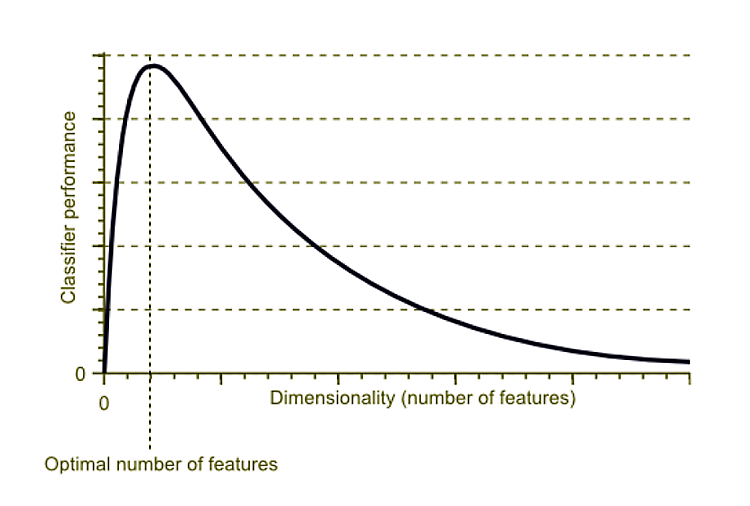
Figure 1: The curse of dimensionality
Feature selection or attribute selection refers to identification of features that are best suited for the creation of a stable predictive model and improve efficiency. This is where a data scientist first earns his money. The requirement being to identify a subset of attributes Xatt = [xt1, xt2, xt3...xtm] from the input dataset X = [x1, x2, x3 … xn] to output set Y = [y1, y2, y3 .. yk], with k being the predicted features or classes. The idea behind feature selection is akin to trying and listening in on a conversation in a noisy environment. This tuning out of noise allows selection of a reduced feature set while allowing for maximum discriminative capability. Sometimes, it is intuitive to identify such attributes, for example, in a dataset capturing operational parameters of an electric motor, the attribute date or plant name may not contribute to the prediction of failure. For situations where identification of contributing attributes is not evident just by examination of the data set, a number of techniques can be utilized. Based on the contribution a feature makes on the prediction of a target, it can be classified as a strongly related, a weakly related, or an unrelated feature.
For example, techniques like localization, stream slicing and annotation is used for models for image or video analytics. For natural language processing (NLP) problems, stop-word removal, information gain (IG), chi-square (X2) and bag-of-words (BOW) can be used. Techniques such as linear discriminant analysis (LDA) , principal component analysis (PCA) and analysis of variance (ANOVA) are useful for handling discrete and time-series data.
Ingestion of irrelevant input features has the dual negative effect of skewing the model by causing it to weigh and include attributes that has little or no significance. For example, for model for classifying titanic survivors the attribute ‘passenger name’ does not provide any insight to the model.
Techniques like F-Test, Forward Selection and LASSO regression can also help evaluate the features by analyzing their relationship and contribution towards a model performance by weighing different subset of features against the target output.
Class representation: One of the key challenges of machine learning is to deal with imbalanced data or frequency bias. In order for a model to be accurate when predicting a class from an input sample, it must be trained with a training set that ensures equal class representation. In an imbalanced or biased dataset, the majority classes dominate minority classes causing the resultant model to be biased towards the majority classes. There are several reasons due to which a data-set could be imbalanced and it usually corresponds to the duration or the manner in which data is collected. Data imbalance is more of a norm rather than an exception as in nature some classes are more prevalent than others, for example, in industry positive (good) samples far exceed negative (defective) samples. As Figure 2 depicts, the reliability of a model is determined by how balanced is the representation of each class in the overall training set.
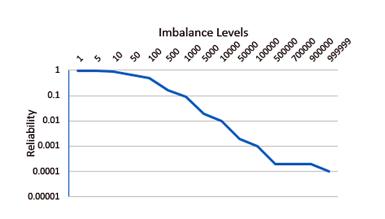
Figure 2: Class imbalance effect on reliability
Intra-class variation: Intra-class variation representation refers to variation of the samples belonging to the same class. For example, for a training dataset used for classifying various types of vehicles, a sample for car can either be red or blue, hatchback or sedan, boxy or curvy, hard-top or convertible etc. This is an extension of the class representation concept discussed earlier. The dataset with adequate variation of classes will improve model efficiency and reduce overfitting within the class. Variation representation will also ensure generalization of model for non-controlled real-world applications. In practice, image augmentation tools and device simulations are used to generate synthetic data covering an array of variations.
The above two topics are key points to consider while assessing the suitability of a dataset for your model. While a high-class imbalance (bias) or a low inter-class variance may cause overfitting of a model and thus lose its ability to generalize, the opposite can cause under fitting and low convergence of a model (See Figure 3). A right balance has to be struck between these topics to optimize the performance of a model.
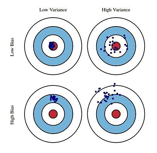
Figure 3: Bias vs Variance
So how do we measure the bias and variance of the data for a model, one way is to compare the prediction accuracy (precision) against the class coverage (recall) during inference and tune the dataset based on the observed results. While precision addresses the question of what percentage of the predictions performed on the validation dataset are actually true, recall indicates how what percentage of the class instances were actually identified. For a model to be efficient it should have both optimal precision and recall.
The calculation of precision is made using the following method:


Where, TP = Total Positives, indicating predictions made correctly; FP = False Positives, and FN = False Negatives, indicating predictions made incorrectly.
Data Cleansing
A dataset collected for a problem may have a lot of impurities. For example, a sensor data stream may include sudden outliers - the cause of which may be a momentary glitch with the sensor or a problem during the transmission or logging of data. For visual data streams data can include background noise, occlusion and/or blackouts. All of these anomalies introduce new features, which are actually irrelevant to the problem a model is designed to address. The objective of data cleansing is to remove impurities, missing values, duplicates or inconsistent data elements. Typically, data cleansing is performed both while training and during inference to prepare the data stream for ingestion.
Removal of noise: Noise refers to a data element, which is inconsistent with the rest of the data stream. Noises doesn't necessarily refer to an outlier data. An outlier can be a data element of a different scale and distance from the rest of the data stream but it still is a valid data item. To illustrate for a data stream on ‘member age’ can include an outlier of 200-cm or of 121-cm to indicate an exceptionally tall or short member, a value of -50-cm or 1500-cm is definitely indicative of noisy data. While noisy elements do not add value to a model, outliers can help make a model more efficient and avoid overfitting. In visual analytics, presence of unrelated features of objects, occlusion, blurry or skewed images can introduce noise in the data stream. Image pre-processing techniques such as morphological operations, localization and segmentation are typically used to remove / suppress undesired features from the input data. Whereas, while performing natural language processing, noise can be reduced by removing extra spaces, punctuation marks, stop words removal, case-correction, spell-check and other impurities. Noise in data-streams can be filtered out by removing of noisy data elements, distance measurements, data filters (e.g. low-pass, Kalman filters, Fourier Transformations) and by interpolation. Incorrect labelling of features can lead to label noise and can negatively influence the efficiency of a model.
Missing data: A data stream may have missing instances due to errors during data capture and processing as a result of manual (missed, ignored) or automated (errors, connectivity loss, glitches) processes (See Figure 4).
Missing values can be categorized in three broad classes, missing not at random (MNAR), missing at random (MAR), and missing completely at random (MCAR). While MAR and MCAR are unexpected losses, MNAR indicates losses due to known issues such as quantization limits. Handling of missing values is based on the data stream properties and can lead to loss of efficiency, bias and overfitting. The way missing data is to be handled is also dependent on the overall data volume as well as what is the degree of sparsity in the dataset. A straightforward method will be to just remove the rows of data that have missing value. This, on the one hand, has the advantage of removing the incomplete rows without injecting simulated or approximated data. On the other, it also has the adverse effect of reducing the dataset and may end up introducing bias if the missing values are from a specific set of classes.
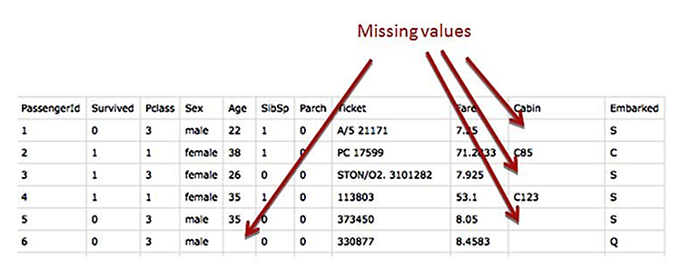
Figure 4: Missing values in dataset
Another way to handle missing data is to just fill in the blanks, but the catch lies in how those blanks are to filled. Since injecting simulated or approximated values can lead to inefficiencies in the model, one has to keep in consideration the weightage those data elements have and the way they are incorporated into the model. The most common approach is to fill the blanks with a mean, median or mode value. For a data element with little or no variance, this may be an “adequate” approach but those elements rarely play a critical role in analysis, as we will discuss later. An alternate will be to apply these factors over a segment of the data element rather than the entire set. This method, although feasible in some scenarios, can miss capturing variations in the data set accurately. For example, it may be possible to fill in missing values from a data element indicating room temperature, as value is not expected to drastically change from sample to sample, but estimation of values from a vibration sensor or an infrared sensor may not be possible to be estimated accurately.
Values can also be estimated using prediction based on earlier values using techniques like regression, K-nearest neighbors, and least mean squared distances. These methods, though more accurate as opposed to the methods discussed earlier, are compute intensive and difficult to implement.
Missing data is also a factor of volume and spread. By spread, we mean how the values missing are spread out across the length of data. For example, sensor glitches or connectivity latencies may cause an occasional drop of value in the stream; typically, these gaps can be approximated using the values that come before or after the missing instance. On the other hand, if successive values from a particular event are unavailable, the prediction of such an event will not be possible by using rest of the stream. In terms of volume, if significant portion of the data is missing, it is prudent to remove that data-stream from analysis or re-inspect the data capture methods. One way to quantify such a loss is to follow Pareto’s 80/20 rule: a loss of more than 20% of the data stream can cause loss of potentially critical samples and may introduce frequency bias.
Feature scaling: Captured data in its raw format may have attribute with varied scales due to varied magnitudes, and differences in measurement units. Machine learning models are typically more focused on variation than on magnitude, for example, an attribute with a small magnitude but high variation can contribute more towards prediction accuracy than an attribute with large magnitude but with low variation. Large variations in magnitude in some attribute as compared to others will cause them to dominate the loss and convergence problems. The objective therefore is to make the model more sensitive to variation than to magnitude.
Rescaling of data seek to neutralize the sensitivity of a model to magnitude and ensure a fair weight distribution amongst the attributes. Typically, feature scaling is more effective with algorithms that use some form of distance measures and are therefore more sensitive to magnitudes, such as KNN, K-Means, SVM and regression models. Classification models are not affected much with scaling as they seek to find what values affect the class of the prediction, that being said, classification model converge more quickly to scaled data than to raw format data as they cause smaller oscillations during optimization.
There are techniques to scale the data, one of the more well-known is Standardization(or Z-Score normalization – See Figure 5) - which scales the attributes so they have properties of normal distribution with a mean of 0 and a standard deviation of 1 by subtracting the value of mean from the attribute and dividing by the standard deviation of the feature.
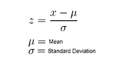
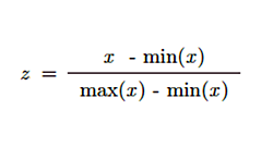
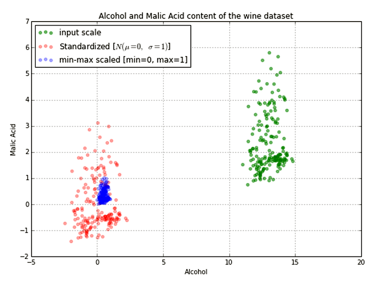
Figure 5: Effect of standardization
The terms feature scaling and feature normalization is used almost interchangeably in several publications. The goal in both cases is to transform data to ensure that relevant features get the desired weightage while analyzing. The difference lies in the approach taken, while scaling uses a somewhat brute-force method to transform the range of data, normalization seeks to transform the distribution of data and describe them as a normal distribution.
There are several other feature-scaling and normalization methods (such as mean normalization, unit vector scaling, softmax, box-cox transformation etc), which can be considered based on the dataset at hand and the use-case being targeted.
In case of deep networks, each layer is affected by variations of all input layers before it hence a minor variation in input parameters gets amplified as we go deeper into the network. Applying feature normalization in such scenarios help reduce internal covariate shift and allows a model converge faster.
Feature engineering: Well-formed features are to a machine-learning model what right proportioned ingredients are to a recipe. Feature engineering is the process of converting raw data to feature vectors suitable for ingestion into a machine-learning algorithm. There are several techniques by which a feature is derived from raw data element. A series of such features makes up a feature vector. Real world data exists in a variety of forms and shapes such as words, numbers, images, sequence and time-series. These data elements are required to be converted into effective feature vectors that can be consumed by a ML algorithm. Feature engineering also seeks to reduce unwanted variations and noise from data samples. This also requires domain knowledge to determine how to effectively represent raw data items into valuable features. Some of the techniques used for engineering are discussed in the ensuing section.
Feature Transformation
Feature transformation is intended to make feature data more suitable for ingestion to a ML model. Consider an example of predicting electricity consumption in a household with room temperature as one of the input features. Although we can easily understand the relation between electricity consumption and room temperature, the input data that may have been collected at per minute interval may not be a suitable form for ingestion due to variations between individual samples and the high volume of distinct samples. Since it is more likely that our goal will be to predict electricity consumption for a month, day of the week or even a time of the day (i.e. morning, afternoon or evening) it would be more effective to take a mean of temperature values for that duration as a representative value. Similarly, we can choose to take max, median or mode as a representative of a subset of data elements based on what we are trying to predict.
Another common technique to transform raw data into usable features is by splitting discrete data values into two or more bins or buckets. Binning or bucketizing as it’s commonly known seeks to categorize a data element based on a class condition. The definition of the class condition depends on the nature of the data column. For example, to represent the success status of an examination result as ‘passed’ or ‘failed’ the class condition would be to compare the actual score against a predetermined passing score. Similarly, while predicting the survival of passengers in the Titanic* dataset using age as a contributing feature, the data elements can be classified as age groups of equal intervals (i.e. 0-10, 11-20,20-30 etc.) or a more general representation of child(0-15 years), young(16-30 years), middle-aged(31-50 years) or old(50-90 years). The bins created can be of unequal interval to avoid over/under representation of a category in an unbalanced dataset.
Techniques such as quantile and decile can be used to split the data into four or ten equal proportion bins.
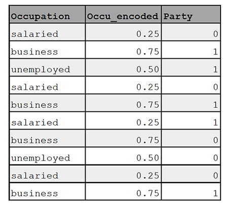
Encoding non-numeric features: Typically, ML models cannot ingest non-numeric data. Feature conversion seeks to represent non-numeric data in numeric form. This allows all attributes to be of the same type and hide unwanted details. Consider a snippet of dataset in the example below, which includes a variety of raw data elements for an individual along with their political leanings.
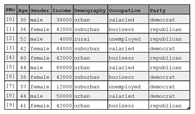
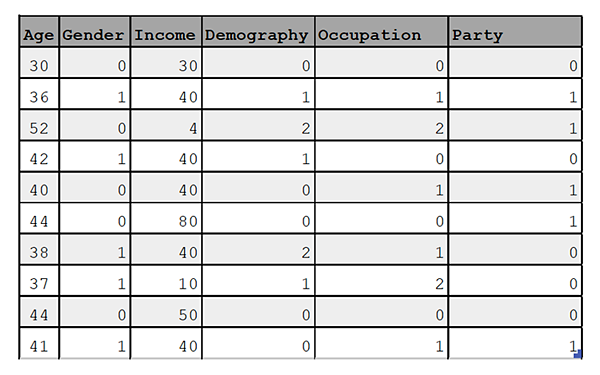
In cases where it is not possible to identify the possible number of encoding classes or categories beforehand, hashing can also be used as a way to assign numeric representation to data.
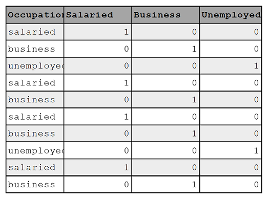
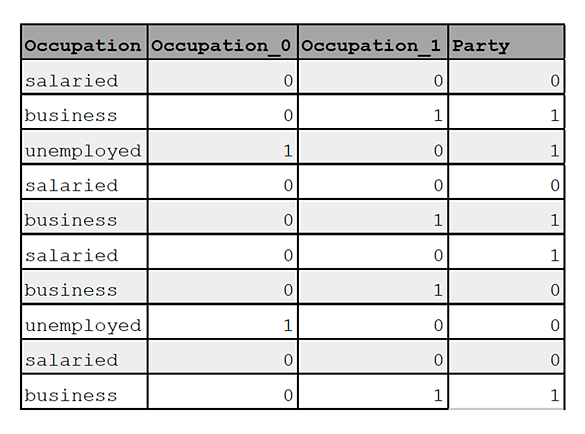
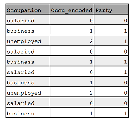
Numerical representation of a categorical feature also needs to reflect whether the categories identified are nominal or ordinal in nature. Nominal categories have values that do not have to adhere to any particular order such as country names or animal names. Ordinal features have values that are relative to each other in the sense that the order of the values matters. One example of this is the size of shirts or age of a person. Encoding nominal features, the same way as ordinal features, has the unfortunate effect of making model attach value to the weight or the amplitude of the feature when none exists. This may result in poor performance. One way to avoid this effect is to transform a feature in a way that assigns equal weight to all values of a feature. One-hot encoding (OHE) is one such technique, which transforms a categorical feature with k possible values to k separate features with binary values. For example, the ‘occupation’ feature in the above dataset can be one-hot encoded as below:
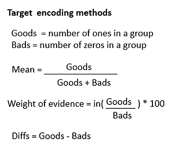
Encoding textual features: Format conversion plays even more important role for text analysis. Unlike numerical data, text data has words with similar meaning, words with multiple meanings, and words that are represented differently in the sentence. Traditional techniques such as ‘one-hot’ encoding is inefficient and largely ineffective in representing approximately 13 million words representations in English vocabulary (other languages may have more). Text processing techniques use word embeddings to represent words; word embeddings represent words as numbers. Some of the more popular methods of extracting word embeddings from text are index-based encoding, Bag-Of-Words (BOW) and Word to Vector (Word2Vector) techniques.
Index-based encoding tries to map each word in a corpus to an index value. A technique like stemming or lemmatization can be used to reduce inflection in words and convert them to their root or stem form before Index base encoding.
The Bag-Of-Words is a fairly simple and flexible technique for extracting features from text. The technique discards any contextual information about the sequence or the order of the words in a sentence (hence the phrase ‘bag’) and attempts to organize words in terms of their count in the samples provided. Each sample is then mapped against this vocabulary of words, the presence or absence of each word is marked with a 1 (presence) or 0 (absence). For example, for a text sample “To be or not to be that is the question”, the BOW vocabulary will look like as below:

Once a complete vocabulary of words from the samples is generated, a sample can be represented by a vector of 1s and 0s of length equal to the total number of words in the vocabulary. For example, the phrase “that is not the question” can be represented as {0,0,0,1,1,1,1,1}. The Continuous bag of words (CBOW) is a model based basic BOW technique that attempts to learn the relationships between sequence of words and predict target words given a context. For example, to predict the next word in a sequence, “The dog chased after the ____.” A Skipgram model, on the other hand, attempts to predict the context for a given word. Typically, output from a CBOW or Skipgram model serves as input for other NLP models.
BOW approach has the limitation of losing the semantic meaning of the word, which may have been used under different context in the document. It also suffers from scalability issues as the generated vector size is directly proportional to the size of the corpus (vocabulary) and may result in sparse vectors, as the absence markers (0s) are considerably more than the presence markers for a large corpus resulting in computational and memory penalties. Variations such as bi-gram and multi-gram BOW representations can help reduce such overheads.
Encoding image data: Encoding Images for ML models typically involves breaking the image components into its color components and converting each component into a two-dimensional vector for ingestion. These are typically augmented by annotations which maps certain regions of the input image to specific labels. While the process is simple and is described by a number of sources for specific AI toolkits, the question of what makes a good image dataset is not frequently discussed. We have talked about the importance of a balanced dataset earlier but there are other parameters also to consider while preparing data for your model. While it seems logical to use higher resolution images for classification, important thing to consider is that at the core of any deep learning model are matrix operations, which are both compute and memory intensive. Hence, there exists a trade-off between what is logical vs what is optimal. Broad features such as shape, color are easier to learn and can be learnt from smaller size images, whereas finer features such as cracks and pits on a surface, hair, small characters etc. require images to have better resolution. Another point to remember is while classifying an object, a model may learn fewer but more important features even though the images are of a smaller size. They end up performing nearly as well and are much faster to train. Most toolkits will also require images of equal size where padding uneven sized images with zeros is helpful. Additionally, as gradient decent is known to favor well-formed features during decision-making, it is advantageous for such features to occupy as much area as possible in a training image set.
Image classification models can also be strengthened by image augmentation to add variation to the image set. This is especially useful in cases where the image set has a smaller number of images or has an unbalanced distribution. Pre-processing training image set to enhance its quality such as diffuse bright light, sharpening, color correction is often to improve model performance but such modifications have an adverse effect of producing good results in ‘lab’ environment while performing poorly in the real world and therefore, must be used carefully and sparingly.
One of the key properties of an image dataset is the color channel used to represent an image. Typical algorithms require each color channel to be processed separately, thereby increasing the dimensionality of the data and the resources required to train a model. The choice of number and type of channel depend on the nature of features being classified. For example, while classifying objects or features where color is an important factor in identification such as classifying fruits, an RGB color representation may produce better results, whereas classifications depending on object brightness may work better by using a representation that separates luminance from chrominance such as YCbCr. Similarly, classifications where the color of the object does not play a significant role such as character recognition, defect detection etc. can be performed with single channel grayscale images, which significantly reduces resource requirement and training time for training a model. Figure 6 is an example of comparative iteration time taken by a simple 3-layer CNN while using 3-Channel RGB images vs 1-Channel grayscale images in the training set.
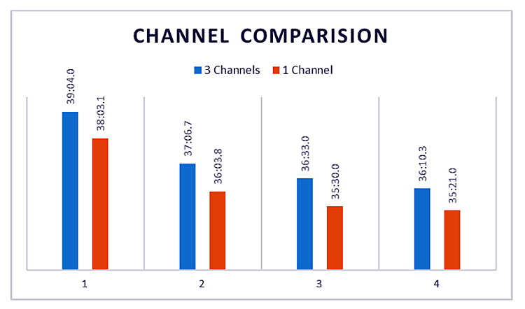
Figure 6: Training time comparison when using 3-Channel vs 1-Channel images
Model accuracy has also been observed to increase when using grayscale images as compared to RGB images.
Goodness of data matters
“Give me six hours to chop down a tree and I will spend the first five sharpening the axe.” -- Abraham Lincoln.
The same can be said about preparing the data for ingestion by an artificial intelligence model. Gathering the right kind and volume of data is the most time-taking task of any data scientist. Like a good recipe, an AI model is only as good as the quality and proportions of its ingredients. Data preparation remains one of the most underrated aspect of machine learning with much of the effort focused on model design and tuning. Goodness of data is directly proportional to the performance of a machine-learning model and hence, is an important part of any AI/ML application.
References
Kuljeet Singh
Kuljeet Singh, in a career spanning 18+ years, has worked extensively in the Internet-of-Things, Artificial Intelligence, Multimedia and Embedded Systems domains. Presently serving as a Solutions Architect (IoT & AI) with Wipro’s Industrial and Engineering Services (IES) division, he is working on the development and deployment of AI/ML based Intelligent IoT edge and gateway platforms. He is also working with the technology teams of leading customers and industry experts on the next generation of IoT and AI solutions. For more information, contact Kuljeet at kuljeet.singh@wipro.com.